Stochastic Numerical Methods for Optimal Voronoï Quantization
Published:
Table of contents
- Introduction
- Voronoï tesselation
- Voronoï quantization
- Optimal quantization
- How to build an optimal quantizer?
- References
Introduction
In this post, I describe the two main Monte-Carlo simulation-based procedures used to build an optimal Voronoï quantizer of $X$. Optimal quantization was first introduced in (Sheppard, 1897), where the author focused on the optimal quantization of the uniform distribution over unit hypercubes. It was then extended to more general laws motivated by applications to signal transmission in the Bell Laboratory in the 1950s (see (Gersho & Gray, 1982)).
Optimal quantization is also linked to an unsupervised learning computational statistical method. Indeed, the K-means method, which is a nonparametric automatic classification method consisting, given a set of points and an integer $k$, in dividing the points into $k$ classes (clusters), is based on the same algorithm as the Lloyd method used to build an optimal quantizer. The K-means problem was formulated by Steinhaus in (Steinhaus, 1956) and then taken up a few years later by MacQueen in (MacQueen, 1967).
In the 90s, optimal quantization was first used for numerical integration purposes for the approximation of expectations, see (Pagès, 1998), and later used for the approximation of conditional expectations: see (Bally et al., 2001; Bally & Pagès, 2003; Bally et al., 2005) for optimal stopping problems applied to the pricing of American options, (Pagès & Pham, 2005; Pham et al., 2005) for non-linear filtering problems, (missing reference) for stochastic control problems, (Gobet et al., 2005) for discretization and simulation of Zakai and McKean-Vlasov equations and (Brandejsky et al., 2012; De Saporta & Dufour, 2012) in the presence of piecewise deterministic Markov processes (PDMP).
First I remind what are a Voronoï tesselation, a quadratic optimal quantizer and their main properties. Then, I explain the two algorithms that were first devised in order to build an optimal quantization of a random vector $X$. All explanations are accompanied by some code examples in Python.
All the code presented in this blog post is available in the following Github repository: montest/stochastic-methods-optimal-quantization
Voronoï tesselation
A Voronoï tesselation (or diagram) is a way, given a set of points (also called centroids) in $\mathbb{R}^d$, to divide / partition a space into regions or cells. For each cell, all the points in it are closer to the centroid associated to the cell than any other centroid.
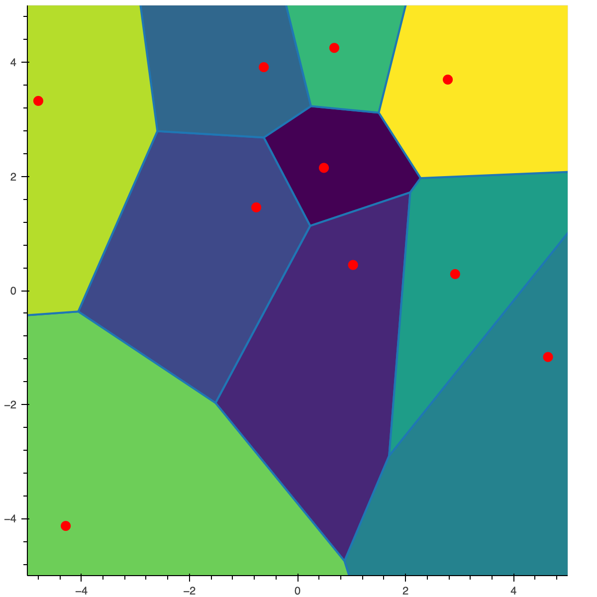
For example, in the figure below, all the points in the top right yellow cell are closer to the centroid (red dot in the middle of the cell) than to any other centroid in the green/blue cells. The yellow cell is called the Voronoï cell of the centroid.
I give below a more formal definition of a quantizer and its associated Voronoï tesselation.
Definition
Let \(\Gamma_N = \big\{ x_1^N, \dots , x_N^N \big\} \subset \mathbb{R}^d\) be a subset of size $N$, called $N$-quantizer. $x_i^N$ is a centroid (red dot in the above figure).
A Borel partition $\big( C_i (\Gamma_N) \big)_{i =1, \dots, N}$ of $\mathbb{R}^d$ is a Voronoï partition of $\mathbb{R}^d$ induced by the $N$-quantizer $\Gamma_N$ if, for every $i \in { 1, \dots , N }$,
\[C_i (\Gamma_N) \subset \big\{ \xi \in \mathbb{R}^d, \vert \xi - x_i^N \vert \leq \min_{j \neq i }\vert \xi - x_j^N \vert \big\}.\]The Borel sets $C_i (\Gamma_N)$ are called Voronoï cells of the partition induced by $\Gamma_N$.
For example, for a list of centroid centroids ( \(\Gamma_N\)) and a given point p, the closest centroid to p can be find using the following method that returns the index i of the closest centroid and the distance between this centroid x_i and p.
from typing import List
Point = np.ndarray

def find_closest_centroid(centroids: List[Point], p: Point):
    index_closest_centroid = -1
    min_dist = sys.float_info.max
    for i, x_i in enumerate(centroids):
        dist = np.linalg.norm(x_i - p)
        if dist < min_dist:
            index_closest_centroid = i
            min_dist = dist
    return index_closest_centroid, min_dist
Voronoï quantization
Now, going back to our initial problem: let $X$ be an $\mathbb{R}^d$-valued random vector with distribution $\mu = P_{X}$ and $\vert \cdot \vert$ be the euclidean norm in $\mathbb{R}^d$.
In simple terms, an optimal quantization of a random vector $X$ is the best approximation of $X$ by a discrete random vector $\widehat X^N$ with cardinality at most $N$.
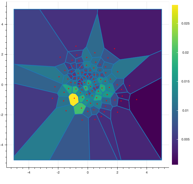
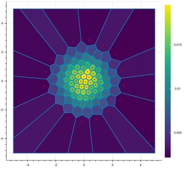
In the following figure, I display 2 possible quantizations of size $100$ of a standard gaussian random vector $X$ of dimension 2. The red dots represents the possible values (also called centroids) of the discrete random vector and the color of each cell represents the probability associated to each value. The figure on the left is a random quantization of $X$ while the figure on the right shows a quadratic optimal quantization of $X$.
Now, let us be a bit more precise and give some definitions of the main notations use in this post.
Definition
A Voronoï quantization of $X$ by $\Gamma_N$, $\widehat X^N$, is defined as nearest neighbor projection of $X$ onto $\Gamma_N$ associated to a Voronoï partition $\big( C_i (\Gamma_N) \big)_{i =1, \dots, N}$ for the euclidean norm
\[\widehat X^N := \textrm{Proj}_{\Gamma_N} (X) = \sum_{i = 1}^N x_i^N \mathbb{1}_{X \in C_i (\Gamma_N) }\]and its associated probabilities, also called weights, are given by
\[\mathbb{P} \big( \widehat X^N = x_i^N \big) = \mathbb{P}_{_{X}} \big( C_i (\Gamma_N) \big) = \mathbb{P} \big( X \in C_i (\Gamma_N) \big).\]Optimal quantization
Now, we can define what an optimal quantization of $X$ is: we are looking for the best approximation of $X$ in the sense that we want to minimize the distance between $X$ and $\widehat X^N$. This distance is measured by the standard $L^2$ norm, denoted $\Vert X - \widehat X^N \Vert_{_2}$, and is called the mean quantization error. But, more often, the quadratic distortion defined as half of the square of the mean quantization error is used.
Definition
The quadratic distortion function at level $N$ induced by an $N$-tuple $x := (x_1^N, \dots, x_N^N) $ is given by
\[\mathcal{Q}_{2,N} : x \longmapsto \frac{1}{2} \mathbb{E} \Big[ \min_{i = 1, \dots, N} \vert X - x_i^N \vert^2 \Big] = \frac{1}{2} \mathbb{E} \Big[ \textrm{dist} (X, \Gamma_N )^2 \Big] = \frac{1}{2} \Vert X - \widehat X^N \Vert_{_2}^2 .\]Of course, the above result can be extended to the $L^p$ case by considering the $L^p$-mean quantization error in place of the quadratic one.
Thus, we are looking for quantizers $\widehat X^N$ taking value in grids $\Gamma_N$ of size $N$ which minimize the quadratic distortion
\[\min_{\Gamma_N \subset \mathbb{R}^d, \vert \Gamma_N \vert \leq N } \Vert X - \widehat X^N \Vert_{_2}^2.\]Classical theoretical results on optimal quantizer can be found in (Graf & Luschgy, 2000; Pagès, 2018). Check those books if you are interested in results on existence and uniqueness of optimal quantizers or if you want further details on the asymptotic behavior of the distortion (such as Zador’s Theorem).
How to build an optimal quantizer?
In this part, I will focus on how to build an optimal quadratic quantizer or, equivalently, find a solution to the following minimization problem
\[\textrm{arg min}_{(\mathbb{R}^d)^N} \mathcal{Q}_{2,N}.\]For that, let’s differentiate the distortion function \(\mathcal{Q}_{2,N}\). The gradient \(\nabla \mathcal{Q}_{2,N}\) is given by
\[\nabla \mathcal{Q}_{2,N} (x) = \bigg[ \int_{C_i (\Gamma_N)} (x_i^N - \xi ) \mathbb{P}_{_{X}} (d \xi) \bigg]_{i = 1, \dots, N } = \Big[ \mathbb{E}\big[ \mathbb{1}_{X \in C_i (\Gamma_N)} ( x_i^N - X ) \big] \Big]_{i = 1, \dots, N }.\]The latter expression is useful for numerical methods based on deterministic procedures while the former featuring a local gradient is handy when we work with stochastic algorithms, which is the case in this post.
Two main stochastic algorithms exist for building an optimal quantizer in \(\mathbb{R}^d\). The first is a fixed-point search, called Lloyd method, see (Lloyd, 1982; Pagès & Printems, 2003) or K-means in the case of unsupervised learning and the second is a stochastic gradient descent, called Competitive Learning Vector Quantization (CLVQ) or also Kohonen algorithm see (Pagès, 1998; Fort & Pages, 1995).
Lloyd method
Starting from the previous equation, when we search a zero of the gradient, we derive a fixed-point problem. Let \(\Lambda_i : \mathbb{R}^N \mapsto \mathbb{R}\) defined by
\[\Lambda_i (x) = \frac{\mathbb{E}\big[ X \mathbb{1}_{ X \in C_i (\Gamma_N)} \big]}{\mathbb{P} \big( X \in C_i (\Gamma_N) \big)}\]then
\[\nabla \mathcal{Q}_{2,N} (x) = 0 \quad \iff \quad \forall i = 1, \dots, N \qquad x_i = \Lambda_i ( x ).\]Hence, from this equality, we deduce a fixed-point search algorithm. This method, known as the Lloyd method, was first devised by Lloyd in (Lloyd, 1982). Let $x^{[n]}$ be the quantizer of size $N$ obtained after $n$ iterations, the Lloyd method with initial condition $x^0$ is defined as follows
\[x^{[n+1]} = \Lambda \big( x^{[n]} \big).\]In our setup, in absence of deterministic methods for computing the expectations, they will be approximated using Monte-Carlo simulation. Let \(\xi_1, \dots, \xi_M\) be independent copies of \(X\), the stochastic version of \(\Lambda_i\) is defined by
\[\Lambda_i^M ( x ) = \frac{\displaystyle \sum_{m=1}^M \xi_m \mathbb{1}_{ \big\{ \textrm{Proj}_{\Gamma_N} (\xi_m) = x_i^N \big\} } }{\displaystyle \sum_{m=1}^M \mathbb{1}_{ \big\{ \textrm{Proj}_{\Gamma_N} (\xi_m) = x_i^N \big\} } }. % \qquad \mbox{with} \qquad \Gamma_N = \{ x_1^N, \dots, x_N^N \}\]Hence, the $n+1$ iteration of the Randomized Lloyd method is given by
\[x^{[n+1]} = \Lambda^M \big( x^{[n]} \big).\]During the optimization of the quantizer it is possible to compute the weight \(p_i^N\) and the local distortion \(q_i^N\) associated to a centroid defined by
\[p_i^N = \mathbb{P} \big( X \in C_i (\Gamma_N) \big) \quad \mbox{ and } \quad q_i^N = \mathbb{E}\big[ (X - x_i^N)^2 \mathbb{1}_{X \in C_i (\Gamma_N)} \big].\]I give below a Python code example for the Randomized Lloyd method that takes as input the quantizer $x^{[n]}$ and $M$ samples $(\xi_m)_{m = 1, \dots, M}$ of $X$ and returns $x^{[n+1]}$, the weights and the local-distortion approximated using Monte-Carlo.
import numpy as np

def fixed_point_iteration(centroids, xs: List[Point]):
    N = len(centroids)  # Size of the quantizer
    M = len(xs)  # Number of samples

    # Initialization step
    local_mean = np.zeros((N, 2))
    local_count = np.zeros(N)
    local_dist = 0.

    for x in xs:
        # find the centroid which is the closest to sample x
        index, l2_dist = find_closest_centroid(centroids, x)

        # Compute local mean, proba and distortion
        local_mean[index] = local_mean[index] + x
        local_dist += l2_dist ** 2  # Computing distortion
        local_count[index] += 1  # Count number of samples falling in cell 'index'

    for i in range(N):
        centroids[i] = local_mean[i] / local_count[i] if local_count[i] > 0 else centroids[i]

    probas = local_count / float(M)
    distortion = local_dist / float(2*M)

    return centroids, probas, distortion
Then, using fixed_point_iteration and starting from a initial guess $x^0$ of size $N$, we can build an optimal quantizer of a random vector $X$ as long as we have access to a random generator of $X$.
Here is a small code example for building an optimal quantizer of a gaussian random vector in dimension 2 where you can select N the size of the optimal quantizer, M the number of sample you want to generate and nbr_iter the number of fixed-point iterations you want to do using M samples each time.
from tqdm import trange

def lloyd_method(N: int, M: int, nbr_iter: int):
    centroids = np.random.normal(0, 1, size=[N, 2])  # Initialize the Voronoi Quantizer

    with trange(nbr_iter, desc='Lloyd method') as t:
        for step in t:

            xs = np.random.normal(0, 1, size=[M, 2])  # Draw M samples of gaussian vectors

            centroids, probas, distortion = fixed_point_iteration(centroids, xs)  # Apply fixed-point search iteration
            t.set_postfix(distortion=distortion)

            # This is only useful when plotting the results
            save_results(centroids, probas, distortion, step, M, method='lloyd')

    make_gif(get_directory(N, M, method='lloyd'))
    return centroids, probas, distortion
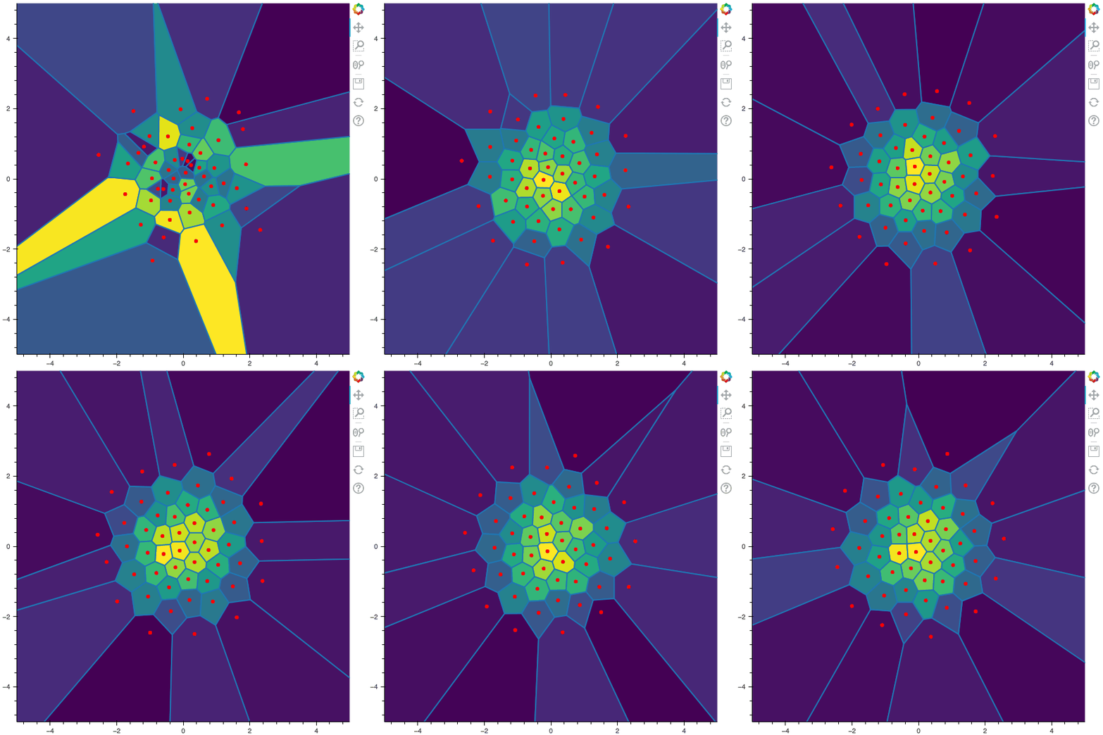
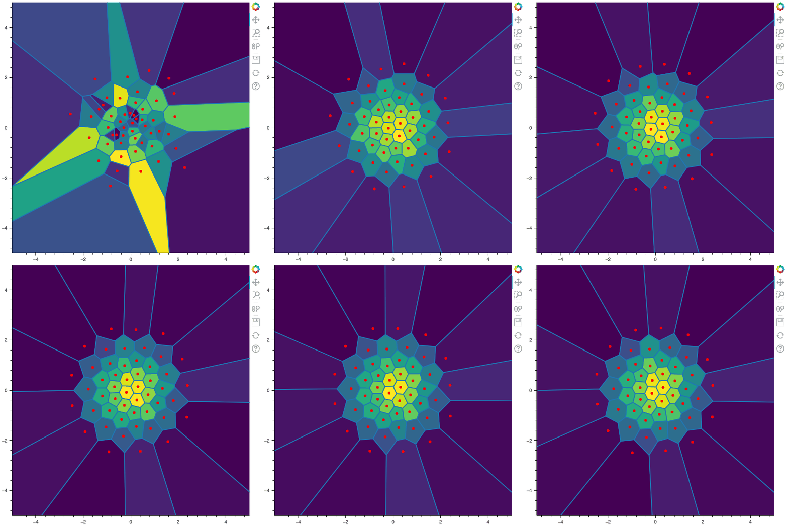
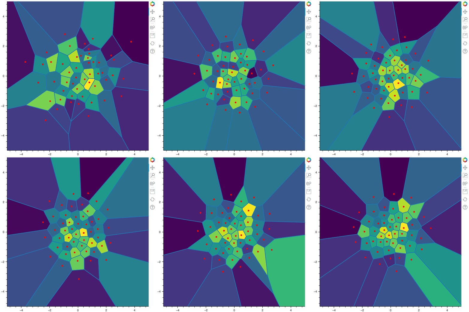
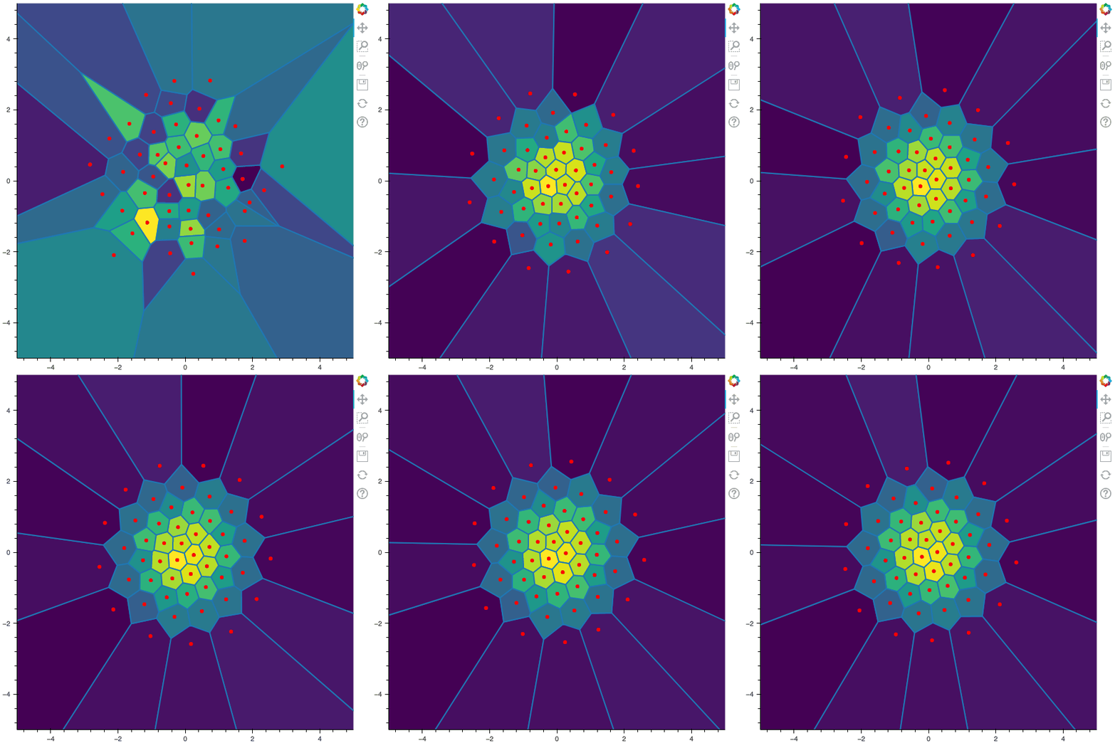
I display below some examples of 100 steps of the Lloyd method applied for a the quantization of size $N$ of the Gaussian Random vector in dimension 2 for different values of $M$. On the left, you can see the 100 iterations of the $N$-quantizer and on the right the distortion computed during the fixed-point iteration.
100 steps of the randomized lloyd method with N=50 and M=5000

100 steps of the randomized lloyd method with N=50 and M=10000 (Click to expand)
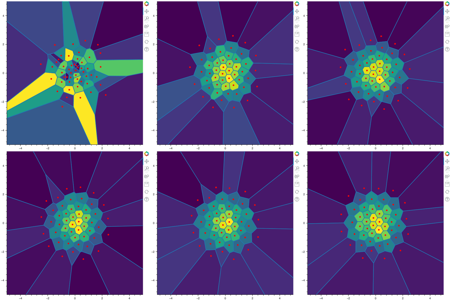

100 steps of the randomized lloyd method with N=50 and M=20000 (Click to expand)
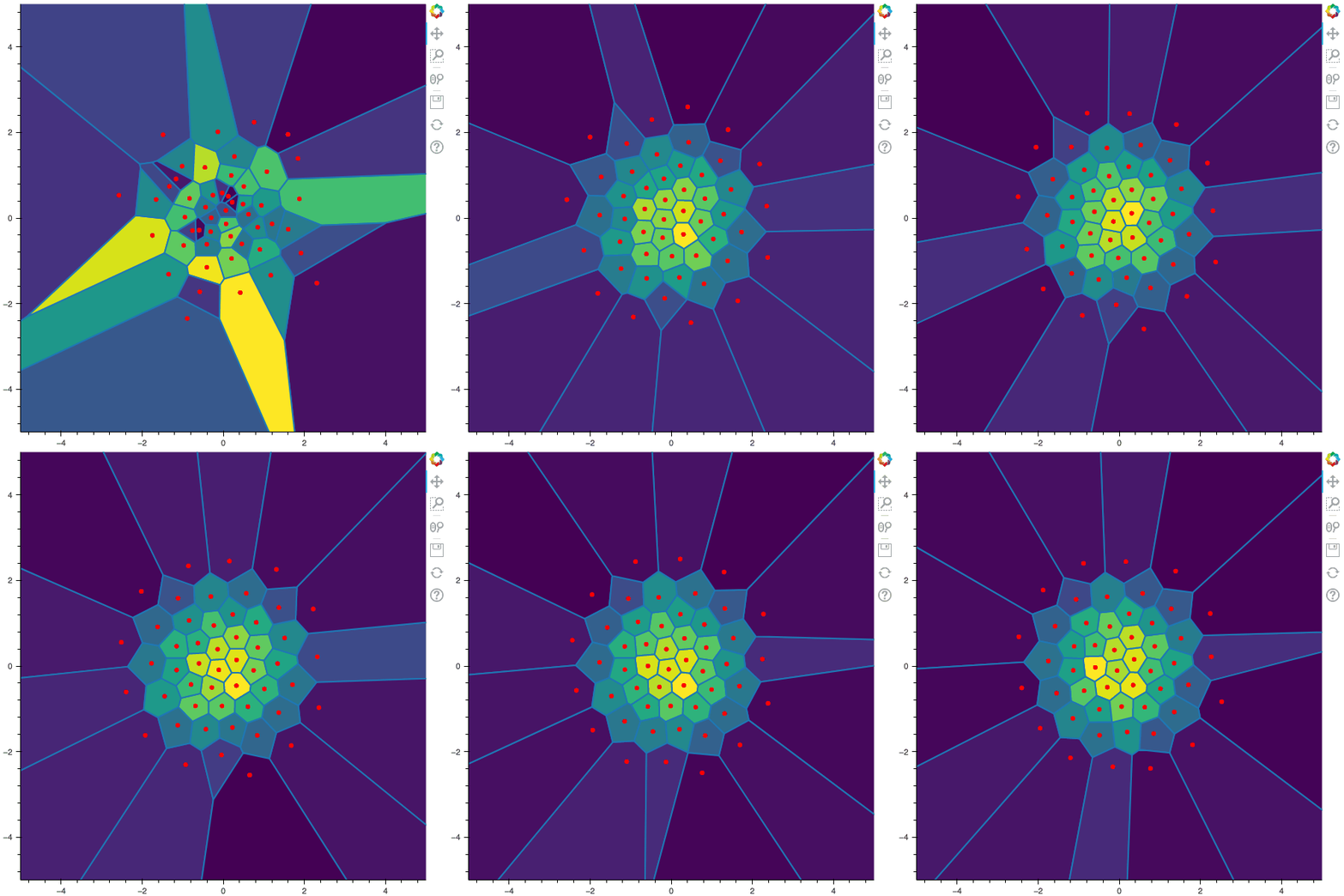

100 steps of the randomized lloyd method with N=50 and M=50000 (Click to expand)
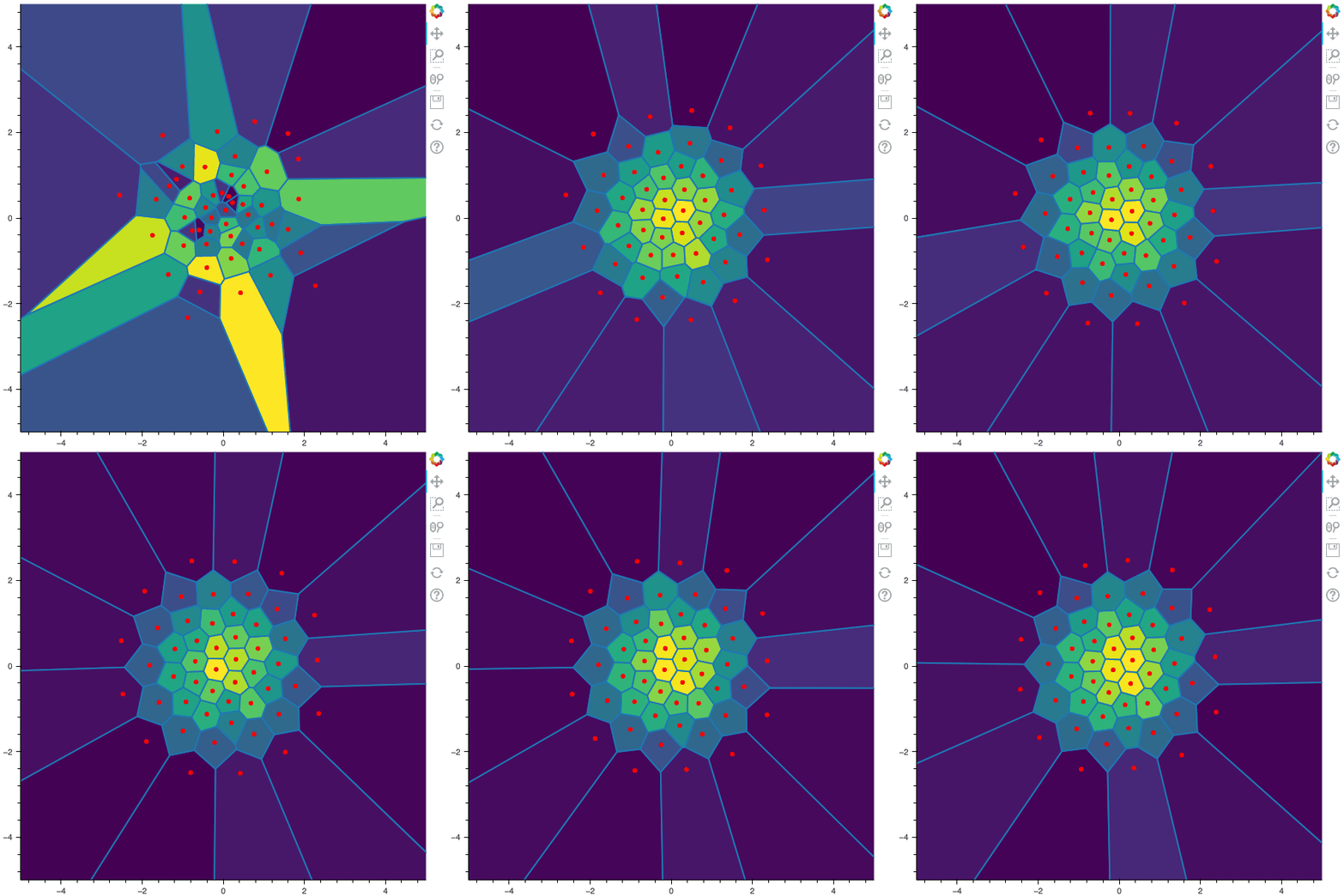

100 steps of the randomized lloyd method with N=50 and M=100000 (Click to expand)

Remark
In the previous code snippet, I use new random numbers, independent copies of $X$, for each batch of size $M$. However, it is also possible to generate only once a set of size $M$ of independent copies of $X$ and then in the loop that iterates nbr_iter times and use them for every batch, as suggested in subsection 6.3.5 of (Pagès, 2018). This amounts to consider the $M$-sample of the distribution of $X$ as the distribution to be quantized. This is stricly equivalent as using the K-means method for clustering the dataset of size $M$ into $N$ clusters.
Competitive Learning Vector Quantization
The second algorithm is a stochastic gradient descent called Competitive Learning Vector Quantization (CLVQ) algorithm, where we use a gradient descent in order to find the grid that minimize the distortion. Since the gradient cannot be computed deterministically, the idea is to replace it by a stochastic version. Let $\xi_1, \dots, \xi_n, \dots$ a sequence of independent copies of $X$, the $n+1$ iterate of the CLVQ algorithm is given by
\[x^{[n+1]} = x^{[n]} - \gamma_{n+1} \nabla \textit{q}_{2,N} (x^{[n]}, \xi_{n+1})\]with
\[\nabla \textit{q}_{2,N} (x^{[n]}, \xi_{n+1}) = \Big( \mathbb{1}_{\xi_{n+1} \in C_i (\Gamma_N)} ( x_i^{[n]} - \xi_{n+1} ) \Big)_{1 \leq i \leq N}\]For the choice on the learning rate I refer to the section 6.3.5 in (Pagès, 2018). Below, you can find a method that returns a learning rate $\gamma_{n+1}$ for a given centroid size N and a step n.
import numpy as np

def lr(N: int, n: int):
    a = 4.0 * N
    b = np.pi ** 2 / float(N * N)
    return a / float(a + b * (n+1.))
Again, during the optimization the weights $p_i^N$ and the local distortions \(q_i^N\) associated to the centroids can be computed. I detail below a Python method that applies M gradient-descent steps of the CLVQ algorithm starting from the init_n iterate $x^{[\textrm{init}_n]}$
def apply_M_gradient_descend_steps(centroids: List[Point], xs: List[Point], probas: List[float], distortion: float, init_n: int):
    N = len(centroids)  # Size of the quantizer

    # M steps of the Stochastic Gradient Descent
    for n, x in enumerate(xs):
        gamma_n = lr(N, init_n+n)

        # find the centroid which is the closest to sample x
        index, l2_dist = find_closest_centroid(centroids, x)

        # Update the closest centroid using the local gradient
        centroids[index] = centroids[index] - gamma_n * (centroids[index]-x)

        # Update the distortion using gamma_n
        distortion = (1 - gamma_n) * distortion + 0.5 * gamma_n * l2_dist ** 2

        # Update counter used for computing the probabilities
        probas = (1 - gamma_n) * probas
        probas[index] += gamma_n

    return centroids, probas, distortion
Hence, starting from a random quantizer of size $N$, the following algorithm will apply n gradient-descent steps of the CLVQ algorithm while ploting the approximated distortion every M steps.
from tqdm import trange

def clvq_method(N: int, n: int, nbr_iter: int):
    M = int(n / nbr_iter)

    # Initialization step
    centroids = np.random.normal(0, 1, size=[N, 2])
    probas = np.zeros(N)
    distortion = 0.

    with trange(nbr_iter, desc='CLVQ method') as t:
        for step in t:
            xs = np.random.normal(0, 1, size=[M, 2])  # Draw M samples of gaussian vectors

            centroids, probas, distortion = apply_M_gradient_descend_steps(centroids, xs, probas, distortion, init_n=step*M)
            t.set_postfix(distortion=distortion, nbr_gradient_iter=(step+1)*M)

    return centroids, probas, distortion
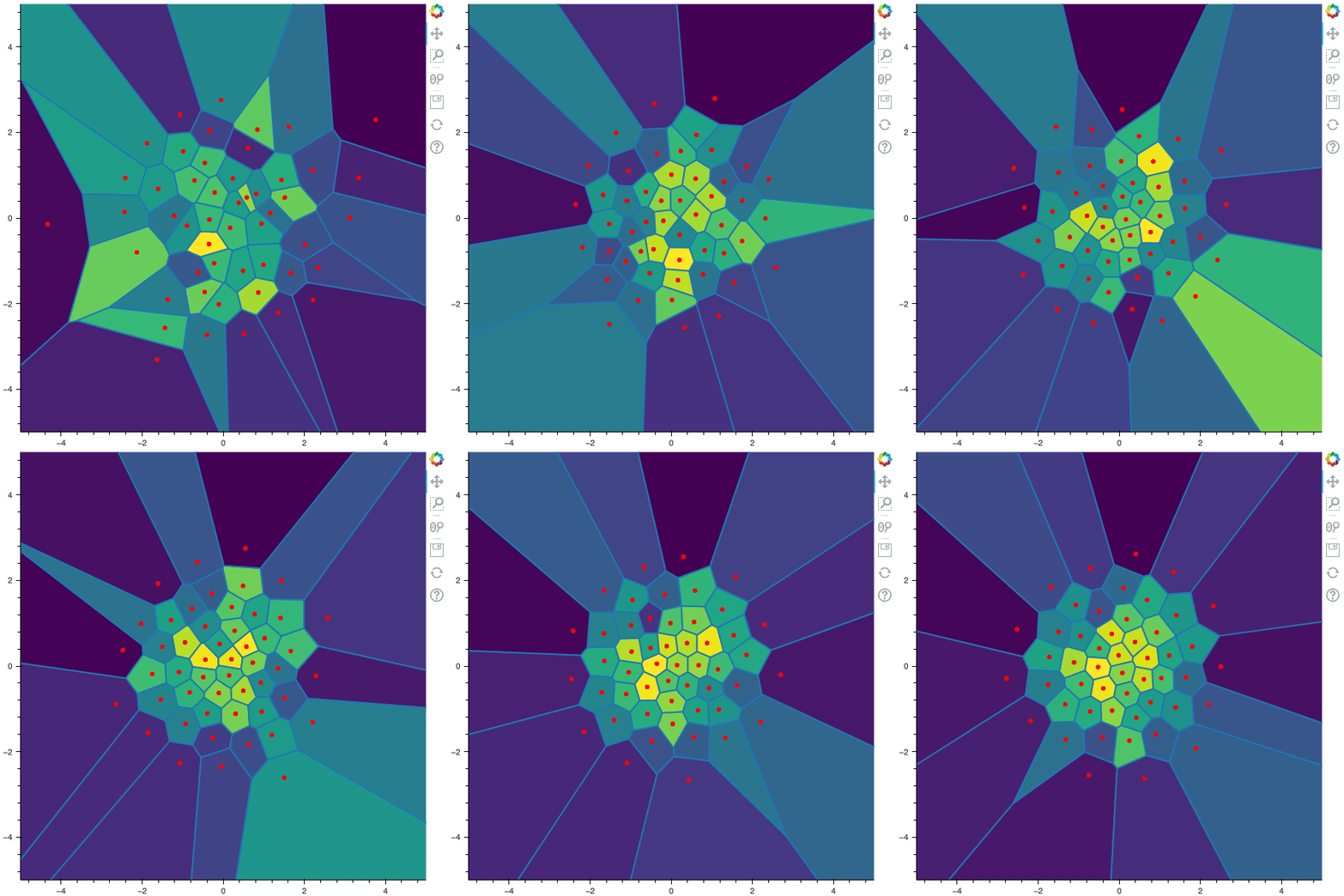
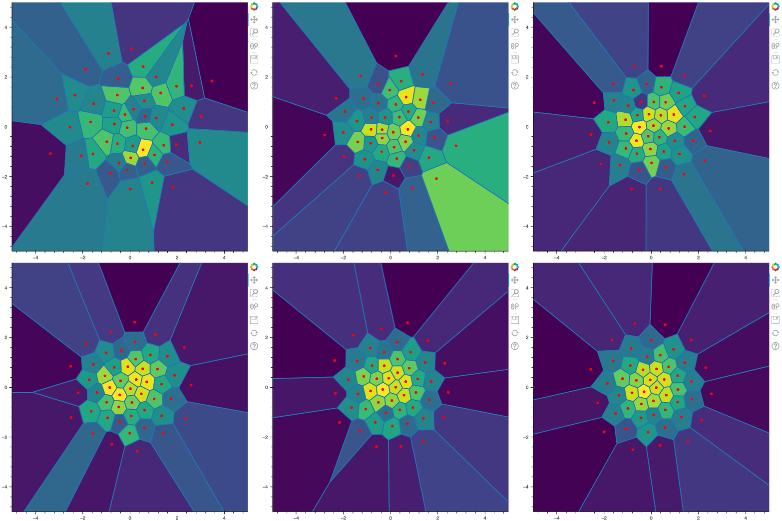
I display below some examples of the CLVQ algorithm applied for a the quantization of size $N$ of the Gaussian Random vector in dimension 2 for different values of $n$ where a plot is made every $n/100$ gradient descent steps. On the left, you can see the 100 iterations of the $N$-quantizer and on the right the distortion.
100 steps of the CLVQ algorithm with N=50 and n=500000

100 steps of the CLVQ algorithm with N=50 and n=1000000 (Click to expand)

100 steps of the CLVQ algorithm with N=50 and n=2000000 (Click to expand)

100 steps of the CLVQ algorithm with N=50 and n=5000000 (Click to expand)
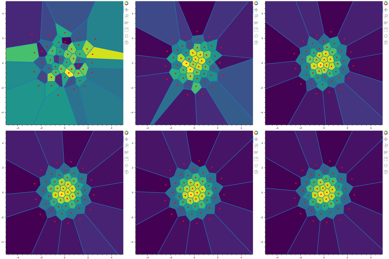

100 steps of the CLVQ algorithm with N=50 and n=10000000 (Click to expand)

Remark
Several developments of the CLVQ algorithm can be considered. For example, I could use the the averaging algorithm of Rupper and Polyak, yielding the averaged quantizer $\widetilde x^{[n+1]}$ defined by
\[\left\{ \begin{aligned} x^{[n+1]} & = x^{[n]} - \gamma_{n+1} \nabla \textit{q}_{2,N} (x^{[n]}, \xi_{n+1}) \\ \widetilde x^{[n+1]} & = \frac{1}{n+1} \sum_{i=1}^{n+1} x^{[i]}. \end{aligned} \right.\]An other possibility would be to consider a batch version of the stochastic algorithm in order to have a better approximation of the gradient at each step, yielding
\[x^{[n+1]} = x^{[n]} - \gamma_{n+1} \frac{1}{M} \sum_{m=1}^M \nabla \textit{q}_{2,N} (x^{[n]}, \xi_{n+1}^m).\]References
- Sheppard, W. F. (1897). On the Calculation of the most Probable Values of Frequency-Constants, for Data arranged according to Equidistant Division of a Scale. Proceedings of the London Mathematical Society, 1(1), 353–380. https://doi.org/10.1112/plms/s1-29.1.353
- Gersho, A., & Gray, R. M. (1982). Special issue on Quantization. IEEE Transactions on Information Theory, 29.
- Steinhaus, H. (1956). Sur la division des corps materiels en parties. Bulletin De l’Académie Polonaise Des Sciences, 1(804), 801. https://doi.org/10.1371/journal.pone.0024999
- MacQueen, J. (1967). Some methods for classification and analysis of multivariate observations. Proceedings of the Fifth Berkeley Symposium on Mathematical Statistics and Probability, 1(14), 281–297.
- Pagès, G. (1998). A space quantization method for numerical integration. Journal of Computational and Applied Mathematics, 89(1), 1–38. https://doi.org/10.1016/S0377-0427(97)00190-8
- Bally, V., Pagès, G., & Printems, J. (2001). A Stochastic Quantization Method for Nonlinear Problems. Monte Carlo Methods and Applications, 7, 21–34. https://doi.org/10.1515/mcma.2001.7.1-2.21
- Bally, V., & Pagès, G. (2003). A quantization algorithm for solving multidimensional discrete-time optimal stopping problems. Bernoulli, 9(6), 1003–1049. https://doi.org/10.3150/bj/1072215199
- Bally, V., Pagès, G., & Printems, J. (2005). A quantization tree method for pricing and hedging multi-dimensional American options. Mathematical Finance, 15(1), 119–168. https://doi.org/10.1111/j.0960-1627.2005.00213.x
- Pagès, G., & Pham, H. (2005). Optimal quantization methods for nonlinear filtering with discrete-time observations. Bernoulli, 11(5), 893–932. https://doi.org/10.3150/bj/1130077599
- Pham, H., Runggaldier, W., & Sellami, A. (2005). Approximation by quantization of the filter process and applications to optimal stopping problems under partial observation. Monte Carlo Methods and Applications, 11(1), 57–81. https://doi.org/10.1515/1569396054027283
- Gobet, E., Pagès, G., Pham, H., & Printems, J. (2005). Discretization and simulation for a class of SPDEs with applications to Zakai and McKean-Vlasov equations. Preprint, LPMA-958, Univ. Paris, 6.
- Brandejsky, A., de Saporta, B., & Dufour, F. (2012). Numerical method for expectations of piecewise deterministic Markov processes. Communications in Applied Mathematics and Computational Science, 7(1), 63–104. https://doi.org/10.2140/camcos.2012.7.63
- De Saporta, B., & Dufour, F. (2012). Numerical method for impulse control of piecewise deterministic Markov processes. Automatica, 48(5), 779–793. https://doi.org/10.1016/j.automatica.2012.02.031
- Graf, S., & Luschgy, H. (2000). Foundations of Quantization for Probability Distributions. Springer-Verlag. https://doi.org/10.1007/BFb0103945
- Pagès, G. (2018). Numerical Probability: An Introduction with Applications to Finance. Springer. https://doi.org/10.1007/978-3-319-90276-0
- Lloyd, S. (1982). Least squares quantization in PCM. IEEE Transactions on Information Theory, 28(2), 129–137.
- Pagès, G., & Printems, J. (2003). Optimal quadratic quantization for numerics: the Gaussian case. Monte Carlo Methods and Applications, 9(2), 135–165.
- Fort, J.-C., & Pages, G. (1995). On the as convergence of the Kohonen algorithm with a general neighborhood function. The Annals of Applied Probability, 1177–1216.

 In this post, I present several PyTorch implementations of the Competitive Learning Vector Quantization algorithm (CLVQ) in order to build Optimal Quantizers of $X$, a random variable of dimension one. In my previous blog post, the use of PyTorch for Lloyd allowed me to perform all the numerical computations on GPU and drastically increase the speed of the algorithm. However, in this article, we do not observe the same behavior, this pytorch implementation is slower than the numpy one. Moreover, I also take advantage of the autograd implementation in PyTorch allowing me to make use of all the optimizers in
  In this post, I present a PyTorch implementation of the stochastic version of the Lloyd algorithm, aka K-means, in order to build Optimal Quantizers of $X$, a random variable of dimension one. The use of PyTorch allows me perform all the numerical computations on GPU and drastically increase the speed of the algorithm.
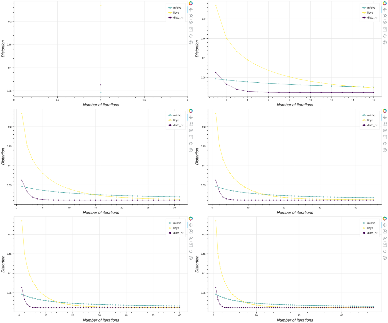 In my previous blog post, I detailed the methods used to build an optimal Voronoï quantizer of random vectors \(X\) whatever the dimension \(d\). In this post, I will focus on real valued random variables and present faster methods for dimension $1$.